In this post, I am going to discuss Deep CorrNet that is described in Correlational Neural Network which is a Common Representation Learning (CRL) technique. I have implemented CorrNet in Python using Keras, Theano as the backend, and Scikit Learn. I have used the same dataset as described in the paper achieving better results across all metrics for transfer learning as well as for data reconstruction. This post covers theoretical as well as step-wise implementation details.

Skip directly to GitHub repository with code.

(For this post I will assume that you are familiar with neural networks, auto-encoders, and Keras. Although this post is self-explanatory, for a detailed explanation please follow these posts: – Implementing neural networks in python, Getting started with the Keras, Building Autoencoders in Keras. )

What is Common Representation Learning?

Common Representation Learning (CRL) is associated with multi-view data – data that can be represented in more than one form/features/view. A common example of multi-view data is movies which are composed of – audio, video, and text (in form of subtitles). Thus, CRL aims to find a combined representation of different modalities of data which is useful for tasks such as classification, clustering, transfer learning, reconstruction, etc. There is a long list of application of CRL – image captioning, visual question answering, video analytics, multi-lingual and cross-language data retrieval, multimedia data analysis, etc.

“The learned common representations can be used to train a model to reconstruct all the views of the data (similar to auto-encoders reconstructing the input view from a hidden representation). Such a model would allow us to reconstruct the subtitles even when only audio/video is available. Now, as an example of transfer learning, consider the case where a profanity detector trained on movie subtitles needs to detect profanities in a movie clip for which the only video is available. If a common representation is available for the different views, then such detectors/classifiers can be trained by computing this common representation from the relevant view (subtitles, in the above example).” – Correlational Neural Networks.

Let’s take an example of image captioning. For the image, we can extract features such as – Histogram of Gradients (HOG), Local Binary Patterns (LBP), Scale-invariant feature transform (SIFT), etc. These days it is common to use a pre-trained model such as AlexNet, VGGNet, Inception module, etc for the feature extraction. Similarly, the caption is represented as one-hot, Word2vec, or GloVe encoding. For this task, CRL can be used to combine word encoding and image features for each image-sentence pair, followed by a scoring mechanism.

In layman’s terms, we can view CRL as – different feature vectors have different dimensions and CRL is a way to combine vectors of varying lengths (since vectors with same dimensions only allow vector operations).

Auto-Encoder

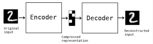
An autoencoder is a neural network that works in two phases:

• In the first phase, the input is encoded to a fixed length vector.
• In the second phase, the model reconstructs the input from the fixed encoded representation. This part is known as the decoding phase.

The above two steps are followed by all auto-encoders.

Correlation Neural Network

Correlation Neural Network or corrnet is an extension to single channel autoencoders. While most autoencoders are single channeled, corrnet can be defined as a two-channel autoencoder where each channel represents a separate modality/view.

What can we do with corrnet?

Before diving into the technical details about the corrnet, let’s see what we can achieve with a 2 – channel autoencoder.

Suppose, we have images along with captions and we train corrnet on these pairs.

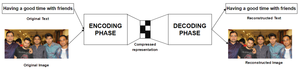
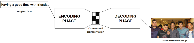
Once trained, the corrnet can be used to generate one view of the data given the other. This is also known as transfer learning. For the above image-text pair, we can even generate an image given a text!

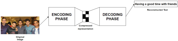
Or, the model can now generate a text corresponding to the given image.

Designing the corrnet

Now, as we have seen what is corrnet capable of, it’s time to design the architecture.

Let the data be given by X for view1 and Y for view2 (in above example X is the text whereas Y is the image). Then the combined representation of data is given by z = (X, Y) (here z = (X, Y) is the concatenated vector representation). The hidden or the compressed representation is computed as

where W is a k × d1 projection matrix, V is a k × d2 projection matrix and b is a k × 1 bias vector. Function f can be any non-linear activation function, for example, sigmoid or tanh. The output layer then tries to reconstruct z from this hidden representation by computing

where W’ is a d1 × k reconstruction matrix, V’ is a d2 × k reconstruction matrix and b’ is a (d1 +d2) × 1 output bias vector. Vector z’ is the reconstruction of z. Function g can be any activation function. This architecture is illustrated in the above Figure.

For each training sample (x_i, y_i), the objective function for the corrnet is designed using following criteria:

• Minimize the self-reconstruction error, i.e., minimize the error in reconstructing x_i from x_i and y_i from y_i.
• Minimize the cross-reconstruction error,i.e., minimize the error in reconstructing x_i from y_i and y_i from x_i.
• Maximize the correlation between the hidden representations of both views.

**NOTE: The cross-reconstruction error is responsible for reconstructing one view of data from the other, while the correlation loss increases the interaction among the two views. 

The final objective function is given as

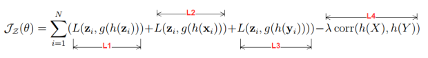
where L1 is the self-reconstruction errors, L2 and L3 are the cross-reconstruction errors, and L4 is the correlation loss. For L2 and L3 the concatenated vector z is obtained by padding 0-vector sequences (will be clear in the implementation section). The authors of CorrNet also introduced a scaling hyperparameter λ. Finally, correlation between two views is computed as

Deep Corrnet

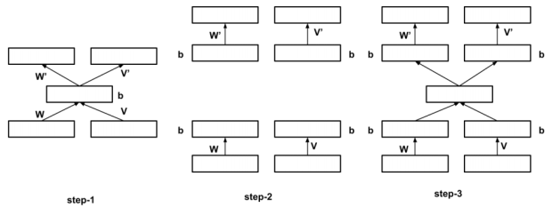
We can also add hidden layers to the corrnet architecture to obtain a deep architecture. The hidden layers are added to the both encoding and decoding phase. This can be done using 3 simple steps as follows:

Implementation

Now, let’s implement the corrnet architecture. The data used in the paper is a modification to MNIST dataset. The dataset has following characteristics:

• Train samples – 60,000
• Test samples – 10,000
• Image size – 28 * 28
• Each image is divided vertically into two halves – left half and right half.
• Dimension of each half – 14 ∗ 28 = 392

Each image is divided into two halves as follows:

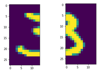
The left half constitutes the first view (X) and the right half is the second view (Y). Thus, our task is to reconstruct one side of the image given the other.

Data loading and pre-processing

data_l = np.load('data_l.npy')
data_r = np.load('data_r.npy')
label = np.load('data_label.npy')

The left viewed images are stored in data_l.npy and right viewed images in data_r.npy. The labels corresponding to each pair is stored in the label which will be used in assessing transfer learning. 

To split the data into training and testing I have implemented a custom split function which works for dividing 2-view data into training and validation sets.

def split(train_l,train_r,label,ratio):
     total = train_l.shape[0]
     train_samples = int(total*(1-ratio))
     test_samples = total-train_samples
     tr_l,tst_l,tr_r,tst_r,l_tr,l_tst=[],[],[],[],[],[]
     dat=random.sample(range(total),train_samples)
     for a in dat:
          tr_l.append(train_l[a,:])
          tr_r.append(train_r[a,:])
          l_tr.append(label[a])

     for i in range(test_samples):
          if i not in dat:
               tst_l.append(train_l[i,:])
               tst_r.append(train_r[i,:])
               l_tst.append(label[i])

     return tr_l,tst_l,tr_r,tst_r,l_tr,l_tst

Now, we can prepare the training and validation dataset using the split function

 X_train_l,X_test_l,X_train_r,X_test_r,y_train,y_test = split(data_l,data_r,label,ratio=0.1)

Encoding Phase

I will use Keras to design the architecture of deep corrnet. The encoding phase is created as

hdim, hdim_deep, hdim_deep2 = 50, 500, 300
dimx, dimy = 392, 392
lamda, nb_epoch, batch_size = 0.02, 40, 100

# input tensor to the model, inpx = view1 and inpy = view2
inpx = Input(shape=(dimx,))
inpy = Input(shape=(dimy,))

# adding dense layers for view1, hx is the hidden representation for view1
hx = Dense(hdim_deep,activation='sigmoid')(inpx)
hx = Dense(hdim_deep2, activation='sigmoid',name='hid_l1')(hx)
hx = Dense(hdim, activation='sigmoid',name='hid_l')(hx)

# adding dense layers for view2, hy is the hidden representation for view2
hy = Dense(hdim_deep,activation='sigmoid')(inpy)
hy = Dense(hdim_deep2, activation='sigmoid',name='hid_r1')(hy)
hy = Dense(hdim, activation='sigmoid',name='hid_r')(hy) 

# at this point we can use a non-linearity for combining hx and hy
# h = Activation("sigmoid")( Merge(mode="sum")([hx,hy]) )
h = Merge(mode="sum")([hx,hy]) # by default the non-linearity is linear

# similarly, non-linearity can be added during decoding phase as well
# recx = Dense(hdim_deep,activation='sigmoid')(h)
recx = Dense(dimx)(h)
# recy = Dense(hdim_deep,activation='sigmoid')(h)
recy = Dense(dimy)(h) 

# creating a intermediate model
branchModel = Model( [inpx,inpy],[recx,recy,h])

Here, branchModel is the intermediate representation of model which will be used during the decoding phase. Please note that I have commented some lines of the code, you can uncomment these line and play around with the model as well.

Creating custom layers in keras

At this point, we need some to create some manual layers in Keras to help us to complete the corrnet architecture.

class ZeroPadding(Layer):
     def __init__(self, **kwargs):
          super(ZeroPadding, self).__init__(**kwargs)

     def call(self, x, mask=None):
          return K.zeros_like(x)

     def get_output_shape_for(self, input_shape):
          return input_shape

class CorrnetCost(Layer):
     def __init__(self,lamda, **kwargs):
          super(CorrnetCost, self).__init__(**kwargs)
          self.lamda = lamda

     def cor(self,y1, y2, lamda):
          y1_mean = K.mean(y1, axis=0)
          y1_centered = y1 - y1_mean
          y2_mean = K.mean(y2, axis=0)
          y2_centered = y2 - y2_mean
          corr_nr = K.sum(y1_centered * y2_centered, axis=0)
          corr_dr1 = K.sqrt(T.sum(y1_centered * y1_centered, axis=0) + 1e-8)
          corr_dr2 = K.sqrt(T.sum(y2_centered * y2_centered, axis=0) + 1e-8)
          corr_dr = corr_dr1 * corr_dr2
          corr = corr_nr / corr_dr
          return K.sum(corr) * lamda

     def call(self ,x ,mask=None):
          hx,hy=x[0],x[1]
          corr = self.cor(hx,hy,self.lamda)
          return corr

     def get_output_shape_for(self, input_shape):
          return (input_shape[0][0],input_shape[0][1])

def corr_loss(y_true, y_pred):
     # this is the loss function for correlation
     return y_pred

If you are not sure about creating custom layers in Keras, then please follow the official documentation (Writing your own Keras layers). The ZeroPadding layer is used to add 0-vector (needed for cross-reconstruction), whereas the CorrnetCost layer is used to add the correlation loss to the final cost function. Finally, corr_loss is the loss function that I will use for CorrnetCost. You can think of this function as a variant of Mean Square Error (MSE), the only difference is that it simply passes the data linearly without doing anything. This is because all the computation for correlation has been carried out in the CorrnetCost layer. So, you might be wondering that why do we need a loss function at all? The only reason I can give is that it is used for completeness, or this is the way Keras works.

** NOTE : The CorrnetCost computes the correlation for the entire batch and therefore we need to do batch normalization to the corrrelation value. This is the reason of setting λ = 0.02, which is low as compared to the original paper. 

I have also included another implementation of CorrnetCost that computes correlation for each sample.

decoding phase

Following our design of corrnet, I have used a combination of 4 types of losses. If you forgot what these loss types are, just take a look at the final cost function in the DESIGNING THE CORRNET section. Please follow the paper for a complete explanation of these losses. Although, in the paper, you will find 8 combinations of losses but the rest are derivative of these four.

# there are 4 loss_types as follows:
# 1 - L1+L2+L3-L4; 2 - L2+L3-L4; 3 - L1+L2+L3 , 4 - L2+L3
loss_type = 2

# reconstruction from view1, view2 = 0-vector
[recx1,recy1,h1] = branchModel( [inpx, ZeroLike()(inpy)])
# reconstruction from view2, view1 = 0-vector
[recx2,recy2,h2] = branchModel( [ZeroLike()(inpx), inpy ])

# reconstruction from combined view1 and view2
[recx3,recy3,h] = branchModel([inpx, inpy])

# adding the correlation loss
corr = CorrnetCost(-lamda)([h1,h2])

# creating the model using different type of losses
if loss_type == 1:
     model = Model( [inpx,inpy],[recx1,recx2,recx3,recy1,recy2,recy3,corr])
     model.compile( loss=["mse","mse","mse","mse","mse","mse",corr_loss],optimizer="rmsprop")
elif loss_type == 2:
     model = Model( [inpx,inpy],[recx1,recx2,recy1,recy2,corr])
     model.compile( loss=["mse","mse","mse","mse",corr_loss],optimizer="rmsprop")
elif loss_type == 3:
     model = Model( [inpx,inpy],[recx1,recx2,recx3,recy1,recy2,recy3])
     model.compile( loss=["mse","mse","mse","mse","mse","mse"],optimizer="rmsprop")
elif loss_type == 4:
     model = Model( [inpx,inpy],[recx1,recx2,recy1,recy2])
     model.compile( loss=["mse","mse","mse","mse"],optimizer="rmsprop")

Here, loss_type = 1 is the design of cost function that uses all four losses, whereas loss_type = 3 and 4 omits the correlation loss. So, you might be wondering how to interpret these combinations of losses. You can think of loss_type = 3 as

Similarly, all other combinations of losses follow the same interpretation.  As there as 4 variables, thus we can have a total of 16 possible combinations of designs for our final objective function.

I have used MSE as the loss function for reconstruction, and Rmsprop as the optimizer.

Training the corrnet

The training of corrnet is dependent on the type of loss that you choose. You can alter the batch size and number of iterations here.

 if loss_type == 1:
      print 'L_Type: l1+l2+l3-L4 h_dim:',hdim,' lamda:',lamda
      model.fit([X_train_l,X_train_r], [X_train_l,X_train_l,X_train_l,X_train_r,X_train_r,X_train_r,np.zeros((X_train_l.shape[0],h_loss))],
                nb_epoch=nb_epoch,batch_size=batch_size,verbose=1)
 elif loss_type == 2:
      print 'L_Type: l2+l3-L4 h_dim:',hdim,' hdim_deep',hdim_deep,' lamda:',lamda
      model.fit([X_train_l,X_train_r], [X_train_l,X_train_l,X_train_r,X_train_r,np.zeros((X_train_l.shape[0],h_loss))],
                nb_epoch=nb_epoch,batch_size=batch_size,verbose=1)
 elif loss_type == 3:
      print 'L_Type: l1+l2+l3 h_dim:',hdim,' lamda:',lamda
      model.fit([X_train_l,X_train_r], [X_train_l,X_train_l,X_train_l,X_train_r,X_train_r,X_train_r],
                nb_epoch=nb_epoch,batch_size=batch_size,verbose=1)
 elif loss_type == 4:
      print 'L_Type: l2+l3 h_dim:',hdim,' lamda:',lamda
      model.fit([X_train_l,X_train_r], [X_train_l,X_train_l,X_train_r,X_train_r],
                nb_epoch=nb_epoch,batch_size=batch_size,verbose=1)

You might need to look for verbose settings. If you see some strange error that halts the training, just set the verbose to 0.

experimentation and results

Now, it’s time for experimentations with the corrnet that we have just created. As per the paper, the evaluation metrics are sum-correlation and transfer learning. I will also use the baselines and results shown in the paper (performance of the compared models). I am using these comparisons just for completeness; the implementation of these compared models is not included in this post.

Compared Models and Baselines

• Canonical Correlation Analysis (CCA)
• Multimodal Autoencoders (MAEs)
• Kernel-based Canonical Correlation Analysis (KCCA)
• Single view (this serve as the baseline for transfer learning)

Evaluation metrics

• Sum-Correlation – It is computed as the total/sum correlation captured in the hidden layer dimensions (hdim = 50) of the common representations learned by the corrnet. Here, we project out the compressed vectors from the trained corrnet. This is essentially the output from the branchModel (defined in the ENCODING PHASE, or you can think of this as the reconstruction from the DECODING PHASE).

def project(model,inp):
     # here, we project out the recontructions from the trained model
     m = model.predict([inp[0],inp[1]])
     return m[2]

def sum_corr(model):
     # the test data is saved in following numpy files
     view1 = np.load("test_v1.npy")
     view2 = np.load("test_v2.npy")

     # cross-reconstruction using the left view only, view2 = 0-vector
     x = project(model,[view1,np.zeros_like(view1)])

     # cross-reconstruction using the right view only, view1 = 0-vector
     y = project(model,[np.zeros_like(view2),view2])

     print "test correlation"
     corr = 0
     for i in range(0,len(x[0])):
          x1 = x[:,i] - (np.ones(len(x))*(sum(x[:,i])/len(x)))
          x2 = y[:,i] - (np.ones(len(y))*(sum(y[:,i])/len(y)))
          temp = sum(x1 * x2)/(math.sqrt(sum(x1*x1))*math.sqrt(sum(x2*x2)))
          corr+=temp
     print corr

• Transfer Learning – To demonstrate transfer learning, the paper follows the task of predicting digits from only one-half of the image. The first step is to learn a common representation for the two views using 50,000 images from the MNIST training data. This is essentially computing the hidden projections (hdim = 50) from the trained model. For each training instance, only one-half of the image is taken which is followed by computation of 50-dimensional common representation using one of the models described above. Finally, I will train a classifier using this representation. For each test instance, I will use only the other half of the image and compute its common representation. This representation is given to the classifier for prediction. According to the paper, I will use the linear SVM implementation as the classifier for all experiments. For all the models considered in this experiment, representation learning is done using 50,000 train images and the best hyperparameters are chosen using the 10,000 images from the validation set. With the chosen model,  5-fold cross-validation accuracy is reported using 10,000 images available in the standard test set of MNIST data.

def svm_classifier(train_x, train_y, valid_x, valid_y, test_x, test_y):
     clf = svm.LinearSVC()
     clf.fit(train_x,train_y)
     pred = clf.predict(valid_x)
     va = accuracy_score(np.ravel(valid_y),np.ravel(pred))
     pred = clf.predict(test_x)
     ta = accuracy_score(np.ravel(test_y),np.ravel(pred))
     return va, ta

def transfer(model):
     # test data is stored in following three files
     view1 = np.load("test_v1.npy")
     view2 = np.load("test_v2.npy")
     labels = np.load("test_l.npy")

     # cross-reconstruction
     view1 = project(model,[view1,np.zeros_like(view1)])
     view2 = project(model,[np.zeros_like(view2),view2])

     perp = len(view1)/5
     print "view1 to view2"
     acc = 0
     for i in range(0,5):
          test_x = view2[i*perp:(i+1)*perp]
          test_y = labels[i*perp:(i+1)*perp]
          if i==0:
               train_x = view1[perp:len(view1)]
               train_y = labels[perp:len(view1)]
          elif i==4:
               train_x = view1[0:4*perp]
               train_y = labels[0:4*perp]
          else:
               train_x1 = view1[0:i*perp]
               train_y1 = labels[0:i*perp]
               train_x2 = view1[(i+1)*perp:len(view1)]
               train_y2 = labels[(i+1)*perp:len(view1)]
               train_x = np.concatenate((train_x1,train_x2))
               train_y = np.concatenate((train_y1,train_y2))

     va, ta = svm_classifier(train_x, train_y, test_x, test_y, test_x, test_y)
     acc += ta
     print acc/5
     print "view2 to view1"
     acc = 0
     for i in range(0,5):
          test_x = view1[i*perp:(i+1)*perp]
          test_y = labels[i*perp:(i+1)*perp]
          if i==0:
               train_x = view2[perp:len(view1)]
               train_y = labels[perp:len(view1)]
          elif i==4:
               train_x = view2[0:4*perp]
               train_y = labels[0:4*perp]
          else:
               train_x1 = view2[0:i*perp]
               train_y1 = labels[0:i*perp]
               train_x2 = view2[(i+1)*perp:len(view1)]
               train_y2 = labels[(i+1)*perp:len(view1)]
               train_x = np.concatenate((train_x1,train_x2))
               train_y = np.concatenate((train_y1,train_y2))
               va, ta = svm_classifier(train_x, train_y, test_x, test_y, test_x, test_y)
          acc += ta
     print acc/5

Accuracy is reported for two settings (i) Left to Right (training on left view, testing on right view) and (ii) Right to Left (training on right view, testing on left view).

Running the corrnet

On running the script (complete script on GitHub) and calling the following modules you can see the performance of corrnet on both of the evaluation metrics.

>>> model,branchModel = buildModel(loss_type = 2)
>>> trainModel(model, loss_type = 2)

Training with following architecture....
L_Type: l2+l3-L4
h_dim: 50
hdim_deep: 500
hdim_deep2: 300
lamda: 0.02

Training done....

>>> testModel(branchModel)

view1 to view2 transfer accuracy
0.8879
view2 to view1 transfer accuracy
0.8964

test sum-correlation
49.1316743225

For the above run, I have used those values of hyperparameters that produced the best results.

comparison with other models

Now, coming to the results analysis, the performance of various models for the task of cross-reconstruction and sum-correlation is given below:

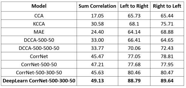
As you can see my implementation of CorrNet achieves the best performance across all 3 metrics. Here, CorrNet-500-300-50 is the configuration with 3 hidden layers with the corresponding number of neurons.

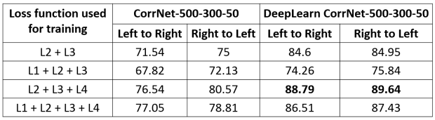
Using different types of losses

Finally, the cross-reconstruction or transfer learning results obtained using different combination of losses is given as

generating images with corrnet

The images reconstructed by the corrnet can be visualized with the help of following functions:

import matplotlib.pyplot as plt

def reconstruct_from_left(model,inp):
     img_inp = inp.reshape((28,14))
     f, axarr = plt.subplots(1,2,sharey=False)
     pred = model.predict([inp,np.zeros_like(inp)])
     img = pred[0].reshape((28,14))
     axarr[0].imshow(img_inp)
     axarr[1].imshow(img)

def reconstruct_from_right(model,inp):
     img_inp = inp.reshape((28,14))
     f, axarr = plt.subplots(1,2,sharey=False)
     pred = model.predict([np.zeros_like(inp),inp])
     img = pred[1].reshape((28,14))
     axarr[1].imshow(img_inp)
     axarr[0].imshow(img)

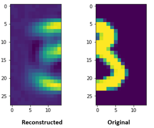
You can see the reconstructed image using the above two functions as

>>> reconstruct_from_left(model,X_train_l[6:7])

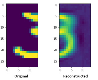
>>> reconstruct_from_right(model,X_train_r[6:7])

What’s next?

So, finally, this long post has come to an end. The idea of reconstruction of data using an unsupervised learning method indeed has its advantages. In my implementation of CorrNet, I have used 2 modifications – using batch correlation, and linear activation during decoding phase. At this point, I can only speculate that these two are the reasons for improved performance. Anyway, I will be looking forward to your feedbacks and questions in the comment section below.

This post explores a glimpse of application of deep learning for CRL. In future posts, I  will present implementation of more research papers focused on CRL, NLP, and CV.